[ML-003] Reinforcement Learning: an Introduction

Reinforcement Learning

Reinforcement learning (RL) is a machine learning technique for solving decision problems by developing an agent that learns from trial-and-error (rewards) by interacting with the environment. Deep reinforcement learning (DRL) is a family of RL methods using deep neural networks.

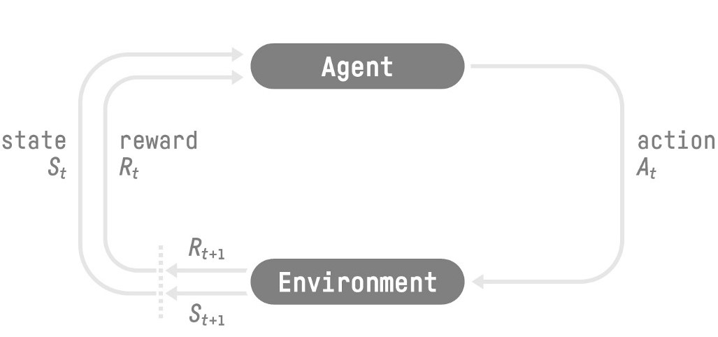
An typical process of RL is shown below (adapted from Sutton and Barto [1]):

RL process from Reinforcement Learning: An Introduction by Richard Sutton and Andrew G. Barto

The basic elements

As shown in the above figure, there are five basic elements defining a RL problem:

Agent: take actions based on the current state (to maximize the expected return or cumulative reward)
Action: the decision made by the agent based on current state
Environment: the world the agent is situated in and interacts with
State: the description of the environment (also called observation)
Reward: the feedback from the environment to the agent after taking some actions

In a time-wise manner, the RL process is a sequence of state, action, reward and next state, denoted as {S_t, A_t, R_t, S_t+1}. The process can be episodic (with a terminal state) or continuous (with no terminal state). This process is Markov, i.e., the future is independent of the past, and thus called Markov decision process (MDP).

The cumulative reward at time step t can be rewritten as:

$G(t) = \sum_{k=0}^{\infty} \gamma^{k}R_{t+k+1}$

where R_t+1 is the instantaneous reward at time t, and γ (in [0,1]) is the discount of future reward.

For episodic RL problems, Monte Carlo learning can be applied by collecting the rewards at the end of the episode; while for continuous RL problems, the temporal different (TD) learning can be applied for rewards estimate.

The classification of RL methods

There are several frameworks to solve a RL problem, from different perspectives. The key solution to the RL problem is to find a good policy to take actions. A policy maps a state to an action the agent is gonna take based on the current state it sees.

The first type is the policy based method, which seeks to find the policy directly. The policy can be determinant, denoted as a=π(s) or stochastic, denoted as π(a|s)=P[A|S], depending on the actions space.

The second type is the value based method, which seeks to find the policy indirectly by finding the maximum reward. The objective is to find a value function (a prediction of future reward):

$v_{\pi}(s) = \mathbb{E}_{\pi}\left [ R_{t+1} + \gamma R_{t+2} + \gamma^2 R_{t+3} + \cdots | S_t =s \right ]$

the action is taken by finding a maximum of ν(s).

There are two types of value functions:

state value function: given a state, find the expected return, denoted as V_π(s) = E_π[ G_t | S_t=s]
(state,action) value function: given a state and an action, find the expected return, denoted as Q_π(s,a) = E_π[ G_t | S_t=s, A_t=a]

The Bellman Equation

The Bellman equation can help update the state-value functions:

$V_{\pi} (s) = \mathbb{E}_{\pi} \left [ R_{t+1} + \gamma V_{\pi} (S_{t+1}) | S_{t} =s \right ]$

and for the action-value functions:

$Q_{\pi} (s,a) = \mathbb{E}_{\pi} \left [ R_{t+1} + \gamma Q_{\pi} (S_{t+1}, A_{t+1}) | S_{t} =s, A_{t} =a \right ]$

For episodic RL problems, Monte Carlo update of value function:

$V(S_t) \leftarrow V(S_t)+\alpha\left [ G_t - V(S_t) \right ]$

and TD update of value function for continuous RL problems:

$V(S_t) \leftarrow V(S_t)+\alpha\left [R_{t+1} + \gamma V(S_{t+1}) - V(S_t) \right ]$

where α is the learning rate. One can see that TD learning has to update the current value until the next state.

Comparison

The link between value and policy is:

$\pi^{*} = \text{arg} \max_{a} Q^{*}(s,a)$

Value based methods are suitable for problems with limited states (low-dimensional space); while policy-based stochastic methods can handle that (high-dimensional space and continuous states).

Value based methods:

Deep Q network
Double DQN

Policy based methods:

policy gradient (gradient ascend)

References

[1] Reinforcement Learning: An Introduction. Richard Sutton and Andrew G. Barto.
[2] Hugging Face tutorial
[3] Medium tutorial